

Previous Article:

In the first three parts of this series, we followed Ethernet frames across a local network, IP packets between networks, and traffic through the Linux networking stack. We now know the machinery behind a network connection. The next challenge is to put those pieces together and build a networked system we can actually test.
The power grid is a network of networks, and software that monitors, operates, protects, or simulates it often has to respect the same boundaries. An application might receive measurements on one interface, exchange information with other devices on a second, and expose a service to a supervisor on a third.
If we want to develop or test such an application, we need an environment that reproduces more than its individual connections. We need the relevant devices, Ethernet segments, routes, and communication paths, together with a way to observe what happens when something changes or fails.
We could build the setup with physical computers, switches, and a router. But even a small test network costs money, takes space, and needs maintenance. Change a requirement, add another device, or investigate a routing problem, and suddenly the environment itself can demand more attention than the software we wanted to test.
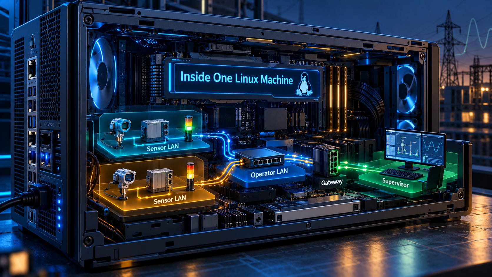
Fortunately, Linux gives us the tools to recreate this kind of topology on a single machine. Network namespaces, virtual Ethernet interfaces, bridges, routing, and NAT let us build realistic communication paths without filling an office with hardware.
In this post you will learn how these pieces fit together by building a small, grid-inspired network. I’ve prepared a hands-on Killercoda course that begins with an empty topology and gradually adds devices, networks, and new requirements.
Open the interactive course: Build an energy network with Linux
The course provides commands, expected observations, and checkpoints. This companion article explains the architecture we are building, why its boundaries matter, and what to look for in the terminal. You can keep it open alongside the interactive lab.
The system we will build
We will start with one local network, add an independent second network, and then introduce communication between devices and a supervisor. Each new requirement will give us a reason to add another piece of Linux networking.
One local network: a measurement becomes an alarm
Imagine a voltage source we want to monitor. We need to read its value, decide whether it has reached an alarm threshold, and show the result on an indicator. To keep the network behavior visible, we will separate those responsibilities into three devices.
We will put three devices on one Ethernet LAN. Let’s call it the Sensor LAN:
A sensor reads the voltage value once per second and publishes the measurement as a Layer 2 multicast message. It reports what it measured; it does not decide whether the value is acceptable.
A logical device listens to the Sensor LAN and compares each measurement with a configured threshold. When the value reaches or exceeds that threshold, it raises its local alarm and publishes an ON command on the same LAN. When the value falls below the threshold, it publishes an OFF command.
An LED with a small controller listens for those commands and turns its indicator on or off. It does not need to know the threshold or repeat the logical device’s decision.
In the lab, three Python programs play these roles. A file stands in for the voltage source, while the LED’s state appears in a log. We use demonstration integers rather than calibrated voltage readings: an input of 5 keeps the alarm clear, while 15 exceeds the threshold of 10.
This gives us a complete path to test: the sensor publishes a measurement, the logical device evaluates it and publishes an alarm command, and the indicator follows that command. The programs publish repeatedly, so we can observe the result both when the value changes and after the system has settled.
All three devices share one Ethernet segment. The measurement and command messages use Ethernet multicast directly, so this first network does not require IP addresses. In a physical setup, we would connect the devices to a switch. In our Linux setup, we will give each device a network namespace, connect it with a veth pair, and use a bridge as the switch.
Multiple local networks: devices share their alarm information
A single LAN is a useful start, but a networked system becomes more interesting when we need to preserve boundaries between independent subsystems.
Suppose we have several voltage sources, each with its own sensor, logical device, and LED. Each subsystem should keep its own Sensor LAN, so a measurement from one does not automatically appear on another. In the course, we will build two of these subsystems.
At the same time, we want the logical devices to know when another subsystem has an alarm. For that, we introduce one additional network: the Operator LAN.
The new requirements are:
Each logical device gets a second network interface. Its first interface stays on its own Sensor LAN; its second connects to the shared Operator LAN.
Each logical device publishes its local alarm state on the Operator LAN. Here it uses an IP multicast message carried over UDP, identifying the device and whether its alarm is ON or OFF.
The logical devices listen for those notifications and store the received alarm information locally. So now each Logical Device contains both types of information: its own state and the alarms from other devices.
For example, Sensor1 reports a high value while Sensor2 remains low. LD1 raises its local alarm, turns LED1 on, and publishes an operator notification. LD2 receives that notification and remembers that LD1 has an alarm, but LD2’s own local alarm stays clear and LED2 remains off.
Notice what has crossed the boundary: information about the alarm. LD1 has received a measurement on one network and created a new message on another. We have not connected the two Sensor LANs into one large Ethernet segment, and Sensor1’s original frame does not travel into Sensor LAN 2.
In a physical setup, these would be distinct switched Ethernet segments, with the logical devices connected to both their local Sensor LAN and the shared Operator LAN. On Linux, we represent them with separate bridges and additional veth connections. The tutorial calls each repeated sensor/device/indicator subsystem a bay.
A supervisor on another network: first routing, then NAT
The logical devices can now exchange alarm information, but operators also need a way to inspect their state from another network.
We will run a supervisor on a different subnet and let it request the status of each logical device. Each response identifies the device, reports its local alarm state, and lists the other device alarms it has heard on the Operator LAN.
For this purpose, each logical-device application also exposes a small TCP status service on its Operator LAN address, using port 10000. The supervisor is on a different subnet, so reaching those services requires a gateway connected to both networks, IP forwarding, and routes for both requests and replies.
First, we will make the connection work with ordinary IP routing. That is enough for the supervisor to reach the devices by their internal addresses. Then we will introduce a separate requirement: give the supervisor stable service addresses on the gateway side, so its configuration does not have to refer directly to each logical device’s Operator LAN address. In this example, destination NAT (DNAT) maps those service addresses to the devices.
In the lab, the mappings will be:
A connection to 192.0.2.10:10000 reaches LD1 at 10.20.0.11:10000.
A connection to 192.0.2.11:10000 reaches LD2 at 10.20.0.12:10000.
These are gateway-owned service addresses on our simulated WAN. We use the documentation prefix 192.0.2.0/24 to represent an external-facing subnet, but every address remains inside the lab. Nothing is exposed to the public Internet.
A physical gateway could perform this translation with destination NAT rules. In the lab, a gateway namespace and iptables do the same job. The supervisor opens a TCP connection to a gateway alias, the gateway rewrites the destination and forwards the packets, and the reply returns through the gateway with the reverse translation applied by connection tracking. Routing still matters, and NAT alone is not a security boundary.
By now, a simple sensor and indicator have grown into a small network of networks: two separate measurement systems, a shared network for device notifications, and another network for supervisory access. That is the complete system we will reconstruct in the hands-on course.
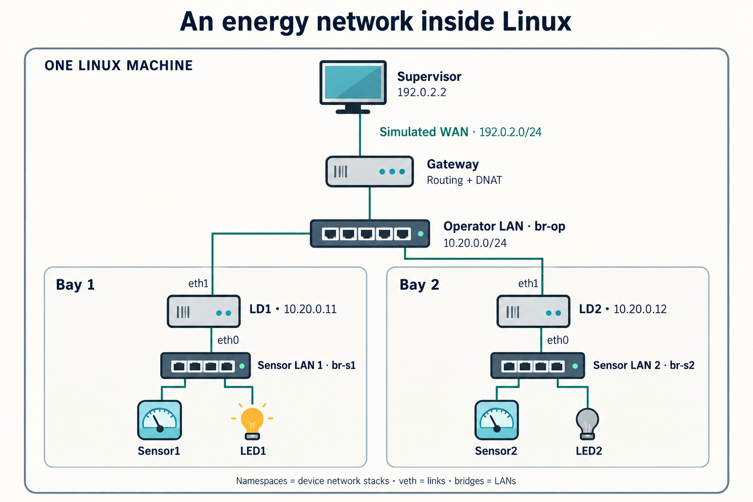
Two separate Sensor LANs connect through their logical devices to a shared Operator LAN. The supervisor reaches device status through a gateway. All connections and devices are represented inside one Linux machine.
The completed topology contains eight device namespaces, three Linux bridges, and a direct veth connection between the gateway and the supervisor. The drawing shows physical and logical connections; application messages can travel in different directions depending on the service.
Here, bay means one repeated sensor, logical device, and indicator subsystem. LD1 and LD2 are small Python applications that play an intelligent-device role; their names do not mean that we have implemented the IEC 61850 logical-device model.
Everything runs on one Linux kernel. The network interfaces, Ethernet switching, IP routing, and packet processing are real Linux mechanisms, while the individual devices, cables, and switches are represented in software.
This is also where the grid connection becomes useful. In a real substation, measurements, device-to-device information, and supervisory communication can have different network boundaries and requirements. Our small model deliberately separates those roles, so we can test communication across the boundaries before introducing actual substation protocols or equipment.
The Linux objects behind the drawing
The course introduces each Linux tool at the moment we need it. Before opening the terminal, it helps to have a mental picture of the objects behind the topology.
A network namespace gives a device its own view of the network stack, including interfaces, routes, neighbor tables, sockets, and firewall rules. Creating a namespace does not automatically connect it to anything. In lesson 1, a new device starts with only a loopback interface.
A veth pair provides two connected virtual Ethernet interfaces. Traffic transmitted from one end arrives at the other. We move one end into a device namespace and usually keep the other as a port on a Linux bridge in the host namespace.
A Linux bridge connects those switch-side ports into one Ethernet LAN. Its forwarding database associates learned MAC addresses with ports. That differs from an IP routing table, which selects the next hop for packets sent between IP networks.
A gateway namespace has an interface in each of two IP subnets. Its presence alone does not make it a router: we must enable IP forwarding and configure the routes that allow the endpoints to exchange requests and replies.
A network namespace is not a virtual machine. It isolates networking resources, not the kernel or filesystem. In this lab, the programs share the underlying kernel and filesystem, so the sensor can read a file you edit from the host shell while using its own isolated network stack. The Linux manual lists the resources isolated by network namespaces.
One detail will prevent confusion during the exercises: host means the disposable Ubuntu machine provided by Killercoda. A command such as ip -n lab-s1 inspects or changes the sensor namespace’s networking state, while ip netns exec lab-s1 ... runs a command inside that namespace. Neither command permanently moves your terminal into the sensor.
How to work through the course
You need basic familiarity with the shell, Python, IP addresses, and switches, plus a general idea of what a substation does. The earlier networking series index provides the networking context, while A Developer’s Map of the European Power Grid provides the wider industry context.
The exercises introduce Linux namespaces from the beginning, so you do not need prior container or IEC 61850 experience.
Plan for roughly 45–60 minutes for the guided path, with more time if you want to experiment. Killercoda environments expire, so keep an eye on the timer and save anything you want to retain.
The ten lessons build the topology in this order:
Lessons What you build and learn 1–3 Separate network stacks, follow both veth ends, and join devices through a bridge. 4 Run the applications, capture Ethernet frames, and trigger a local alarm. 5–6 Repeat a bay, preserve its LAN boundary, and exchange operator notifications. 7–8 Cable another subnet and make requests and replies cross the gateway. 9 Assign gateway aliases and capture packets before and after DNAT. 10 Break a link and a return route, diagnose the failures, and restore the system.
Wait for Ready before starting the first lesson. Setup installs the required tools and places the example programs in /root/energy-lab; you create the networking connections yourself.
Follow the command blocks in order, compare the result with the expected observation, and try to predict what will happen before running the next command. Use Check at the end of each lesson. A successful check confirms the required state, but it cannot confirm that you understand why the network behaves that way. Try explaining each packet path in your own words.
One sequencing detail is worth mentioning: lesson 4 prepares LD1’s operator interface because the supplied program expects both interfaces when it starts. That interface does not connect to the shared Operator LAN until lesson 6.
In Killercoda, going back to an earlier lesson does not undo the commands you have already run. If you see “File exists,” inspect the existing object before repeating a creation command. For a fresh start, the supplied lab.sh reset command clears the lab topology and application state so you can rebuild from lesson 1.
If you want to work without the online timer, the closing lesson explains how to prepare the same files in a disposable Ubuntu 24.04 virtual machine.
What to take from the lab
By the end of the course, you should be able to look at a topology and decide which devices need independent network stacks, which interfaces belong to the same Ethernet segment, and which communication paths require routing.
More importantly, you should be able to distinguish three very different operations: a bridge forwarding an Ethernet frame, a router forwarding an IP packet, and an application receiving information and creating a new message.
The example deliberately uses simple protocols to make network behavior easier to observe. It does not implement IEC 61850 GOOSE, Sampled Values, MMS, or a production SCADA service. The sensor reads demonstration integers, the LED records software state, and alarm notifications have no authentication, persistence, or expiry. The lab also cannot reproduce physical-link timing or protection-system performance.
What it does give us is a way to make the network underneath an application visible and testable, instead of treating interfaces, switching, and routing as an invisible dependency.
Before finishing, try one exercise without step-by-step instructions: draw a third bay before writing any commands. Give it a separate Sensor LAN and connect its logical device to the Operator LAN. Predict which devices should receive its alarm notification and which LEDs should remain unaffected. Then build it, capture the traffic, and compare the result with your prediction. The supplied helper manages two bays, so you will need to launch any additional roles explicitly.
From a Packet to a Networked System
In Part 1, we started with two machines on the same local network. Before they could exchange an IP packet, we needed to understand Ethernet frames, MAC addresses, switches, and ARP. In Part 2, we moved the destination beyond the local network and introduced IP addressing, routing tables, and gateways. We saw that the IP destination describes where the packet is going, while Ethernet handles delivery over each local link.
In Part 3, we turned our attention to the Linux host itself. We followed incoming traffic from the network interface and driver through the kernel networking stack to the application. The socket was no longer just an API call. It was the end of a journey through real operating-system machinery.
And in this fourth part, we have used those ideas to build a small network of networks on one Linux machine. We created interfaces and links, kept local networks separate, connected applications across them, and watched how routing and NAT affected communication. We also introduced faults, because understanding a network means knowing how to investigate it when something stops working.
In this series I wanted to understand what happens beneath networked software well enough to investigate and understand, build and create more complex systems myself. This is still a foundation, not a production substation design. We have deliberately left industrial protocol behavior, redundancy, time synchronization, and security requirements for later. But now we can approach those subjects with a working model of the network underneath them. The next step is to use that model to understand how substations, IEC 61850, IEC 60870-5-104, and SCADA systems actually communicate.
Series Hub:
Networking Machinery for Software Engineers

I have worked with networked software for years, but for most of that time the network was something I used rather than something I really understood. I could open a socket, call an API, connect to an IP address, and continue with the part of the system I was responsible for.