

Previous part:

Intro
The core purpose of a network is to establish communication between multiple nodes. That is already a difficult problem in almost any system, and it becomes even more demanding in critical real-time systems such as the power grid.
But some of the hardest networking problems do not happen between different devices at all. They happen inside one single machine.
It is easy to imagine that once an Ethernet frame reaches the network interface, most of the work is already done and everything after that is trivial. It is not. Behind the black box that we casually call the Linux networking stack is another complex system, with its own objects, queues, memory, control paths and state transitions. This is the system I want to open in this part.
Why should we care about what happens inside one machine? Because some of the most difficult, bug-prone and timing-sensitive problems I have faced were not hidden in the coordination of a huge number of servers or in enormous traffic volumes. They were hidden inside one particular computer that had to process network traffic with extremely strict timing requirements, where a lot could go wrong at very different levels.
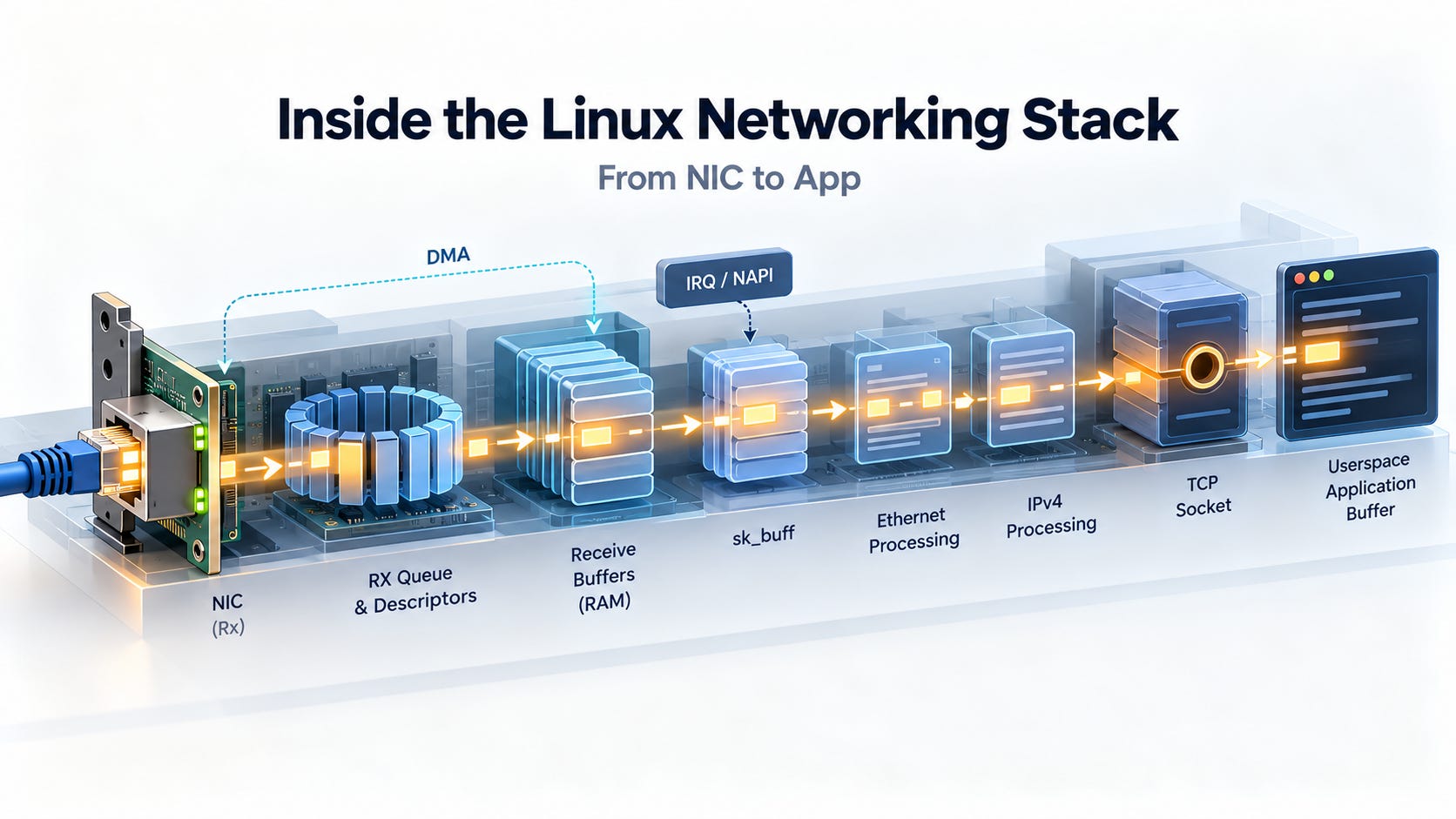
So now I want to open one of the most underestimated black boxes we constantly depend on when working with networked systems: the Linux networking stack.
The route
I tried several ways to explain the whole concept, and the approach I want to use now is the one I wish I had when I first faced this topic. Instead of showing isolated diagrams, we will keep the state of the whole system visible at the same time. We will see userspace, kernel state, memory structures and the communication between them while one simple story evolves.
We will start before our tracked network interface exists in the kernel. Then we will watch Linux discover and initialize the NIC, create the interface representation, prepare the receive path, configure the interface, and finally trace one single Ethernet frame from the cable to a userspace application.
In this post we will discuss the Linux networking stack by following one machine as its networking state evolves. Instead of describing every observable value twice, we will use two languages in parallel: the text will explain why a transition happens and what it means, while the dashboard will show what exists now, what changed, which command was executed, and what the system returned. Long-lived state such as net_device, routing state and the RX machinery will stay in fixed places, while transient objects such as sk_buff will appear only when they actually exist.
There is one deliberate simplification. We follow one physical NIC and the Linux interface that represents it. State 0 therefore shows our tracked net_device, RX queue and routes as absent even though a real Linux system can already contain other interfaces, especially loopback. The goal is to make the birth and evolution of this particular interface visible without pretending that the rest of the operating system does not exist.
Main concepts and characters
Before the actual journey starts, we need a small vocabulary. The important point is that not everything in the diagram belongs to the same category. Some things are regions, some are long-lived objects, some are transient packet objects, and some are mechanisms that connect them.
Regions
Hardware is where the physical NIC, PHY, firmware and hardware buses live. Hardware can read and write selected areas of RAM through DMA and can notify the CPU through interrupts.
Kernel is the privileged part of the operating system. For our story it contains the network driver, interrupt handling, NAPI receive processing, the networking stack, sockets, routing state and kernel objects such as net_device and sk_buff.
Userspace is where normal processes run. This includes applications and tools such as NetworkManager, ip, nmcli and ethtool.
Actors and control interfaces
NIC is the physical network interface controller. It receives frames from the link and cooperates with the driver through queues, descriptors, DMA and interrupts.
CPU executes the kernel and userspace code involved in our story.
Driver is kernel code that knows how to control a specific NIC. It creates and configures much of the receive machinery that we will watch appear in the dashboard.
Netlink is an important message-based interface between userspace and kernel subsystems. Networking tools can use it to request configuration changes or query state, and the kernel can also send notifications back to userspace. In the visualization, Netlink is better represented as a message channel or event log than as a permanent state object.
There is not one single Linux networking tool because there is not one single level of networking state.
ip is the most direct tool in our story for inspecting and changing current kernel networking state. It works with objects such as links, addresses, routes and neighbors, mainly through rtnetlink. When we run ip link or ip route, we are asking what the kernel believes right now, or asking it to change that current state.
NetworkManager is a long-running userspace daemon that sits one level higher. It keeps connection profiles and policy, decides which configuration should be active, and then applies that configuration to the kernel. It can manage addresses, routes, DNS, autoconnect behavior and many device settings. This means NetworkManager has its own idea of what the machine should look like, while the kernel contains what is actually active at this moment.
nmcli is the command-line client for NetworkManager. It does not configure the driver directly. It talks to the NetworkManager daemon over D-Bus, and NetworkManager then uses Netlink and other kernel interfaces to apply the requested configuration.
ethtool looks lower in the stack. It focuses mostly on NIC and driver properties such as link modes, channels, ring sizes, offloads, interrupt coalescing and hardware statistics. Modern ethtool operations use an ethtool Generic Netlink family, while some older operations still use legacy ioctls.
So these tools do not control separate networks. They give us different views and control points over the same running system. ip is close to current kernel network state, nmcli works through NetworkManager’s managed configuration and policy, and ethtool focuses on the device and driver layer. Their responsibilities can overlap, which is exactly why it is useful to keep all of them visible in the same story.
Persistent kernel and memory state
net_device is the central kernel representation of a network interface. It is long-lived relative to individual packets and contains or references interface state such as the interface identity, flags, MTU, queue configuration and driver operations.
RX queue is a logical receive path associated with the NIC and driver. For this visualization, each RX queue will own or reference the receive resources used to process incoming traffic.
RX descriptor ring is a circular array of descriptors shared conceptually between the driver and the NIC. A descriptor does not store the complete Ethernet frame itself. Instead it describes a receive buffer and carries metadata and ownership or completion information that lets the NIC and driver coordinate packet reception.
Receive buffers are areas of RAM prepared for incoming packet data. RX descriptors point to, or otherwise identify, these buffers so that the NIC can DMA frame data into them.
Routing and forwarding state is separate kernel networking state. It is not a field inside net_device. Linux organizes routes in routing tables and uses this information through its FIB, Forwarding Information Base, when making forwarding decisions. Routes describe how destinations should be reached and may reference a network interface, next hop, scope and other routing information. In the dashboard we will show the routes relevant to our tracked interface so commands such as ip route have visible kernel state to inspect.
Transient packet state
sk_buff is Linux’s central packet representation while network data moves through much of the kernel networking stack. It contains metadata and references to packet data. It should be treated very differently from net_device: net_device belongs to the machine, while sk_buff belongs to a particular packet processing episode.
Mechanisms and events
DMA, Direct Memory Access, allows the NIC to access DMA-mapped memory without the CPU copying each byte itself. During receive processing, the NIC can write the incoming frame into a prepared receive buffer in RAM.
IRQ, Interrupt Request, is a hardware notification mechanism. For our story, the NIC can signal that receive work is available. The CPU then runs the interrupt handling path registered by the driver. With NAPI, the interrupt handler typically does not perform the whole receive path itself; it arranges for receive polling to continue in the appropriate kernel context.
Before anything moves: State 0
This is the deliberately empty state from which the story begins. The physical NIC exists in the machine, but Linux has not yet created the kernel representation and receive resources that we want to watch appear.
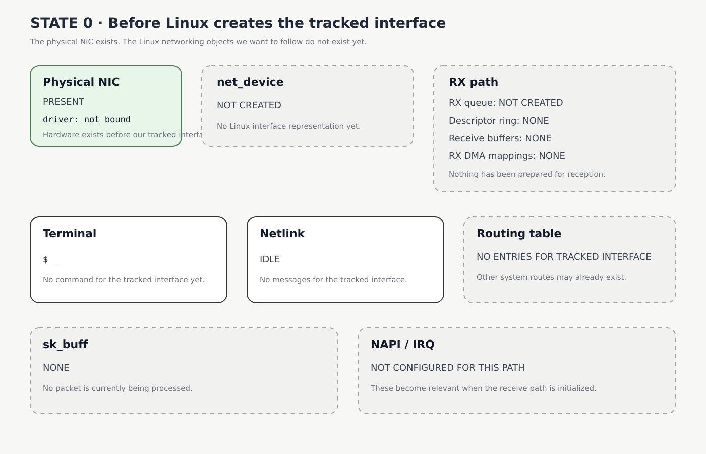
State 0. Initial dashboard. The physical NIC exists, while the tracked net_device, RX queue, receive resources, routing entries and sk_buff are deliberately absent. The Terminal and Netlink panels are idle.
From this point on, the dashboard itself is the state description. Empty panels remain visible as NOT CREATED, NONE or NO ENTRIES, because seeing an object appear is part of the explanation. When a field changes, we will change it there instead of repeating the same information in a table below the image.
Now we can finally change something. The first transition happens when Linux discovers the NIC and the driver introduces it to the networking subsystem.
State 1: the NIC becomes a Linux network interface
The next transition starts when the system boots or the NIC is hot-plugged. Linux discovers the PCI (Peripheral Component Interconnect) device, matches it with the appropriate driver, and invokes the driver’s probe() callback. probe() is the driver’s initialization function for that device. It is where the driver starts setting up the hardware and creating the kernel-side structures needed to use it.
Inside that initialization path, the driver prepares access to the hardware, including mapping the device registers it needs to communicate with the NIC. It also creates its own internal state. The important moment for us comes when the driver creates and registers a net_device.
This is the point where our NIC stops being merely a piece of detected hardware and becomes a network interface that the Linux networking subsystem can work with.
When we say that the driver maps device registers, we are talking about the hardware control registers that the driver needs to access. On a typical PCI NIC this is commonly done through MMIO, memory-mapped I/O. MMIO lets device registers be accessed through addresses handled by the kernel’s device I/O APIs. Linux device I/O documentation
State 1 dashboard
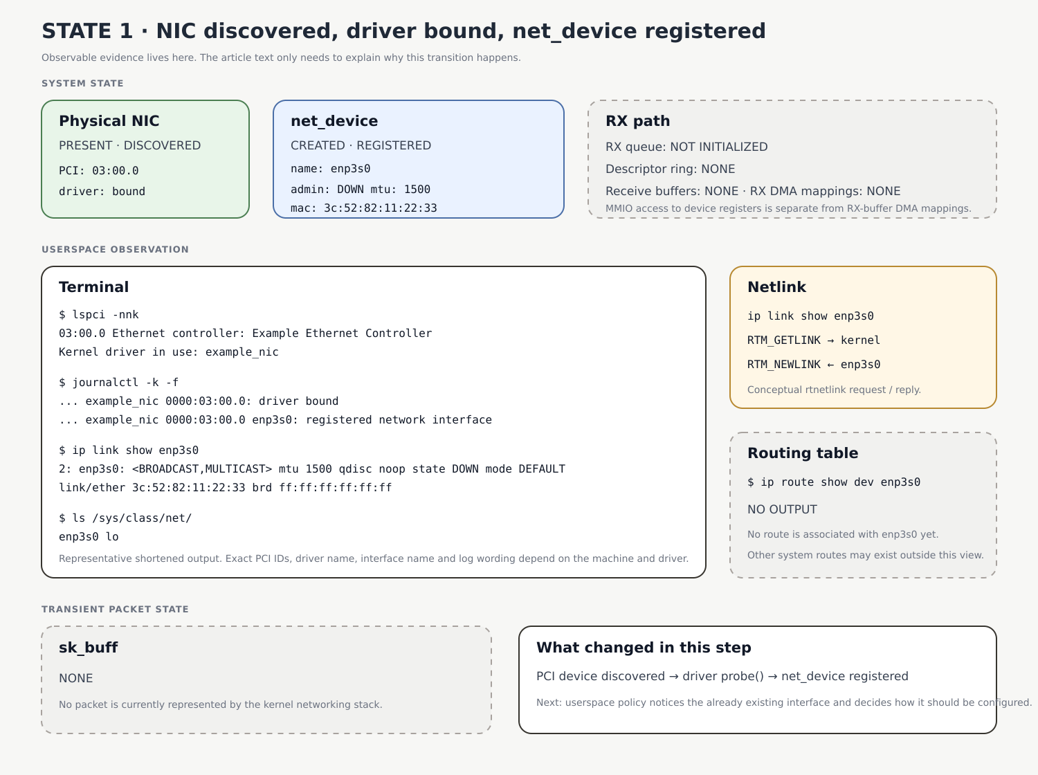
State 1. The dashboard now carries the observable evidence: PCI and driver visibility, kernel log output, the registered net_device, ip link output, sysfs visibility, the rtnetlink request and reply, and the still-empty RX, routing and packet state.
The important part is why this visual change matters. Registering net_device creates the kernel object that the rest of Linux networking can now refer to. Before this moment we had discovered hardware and a bound driver; after it we have a network interface as far as the networking subsystem is concerned.
That gives us the next natural question: what happens when userspace notices the new interface? NetworkManager can now discover the interface and build its own higher-level view of the same device, which gives us the first chance to compare current kernel state with managed userspace configuration.
State 2: NetworkManager discovers the interface
The kernel now has a real network interface called enp3s0, which means userspace services that monitor Linux networking can learn about it too. NetworkManager maintains its own higher-level model above the raw kernel state, so when it discovers the new interface it first decides whether the device should be managed and then looks for connection profiles that can be used with it.
For our story, we will assume that NetworkManager finds a saved Ethernet profile and that the profile is eligible for autoconnect. Autoconnect does not mean that the interface is already connected. It means that NetworkManager is allowed to activate that profile automatically when a suitable device becomes available. NetworkManager autoconnect documentation
We will freeze the system for one conceptual frame before that activation happens. The kernel-side interface is therefore almost exactly where we left it in State 1. What has changed is the userspace management state: NetworkManager now knows about enp3s0, considers it managed, and has a profile it could apply.
State 2 dashboard
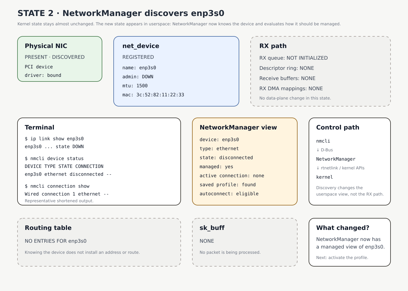
State 2. The kernel interface is still down and the RX, routing and packet state remain unchanged, but NetworkManager now has its own managed view of enp3s0. The terminal compares the kernel view from ip with the higher-level device and profile view from nmcli, while the control panel shows that nmcli talks to NetworkManager over D-Bus rather than directly to the kernel.
This is the first point where two related views of the same interface exist at the same time. The kernel owns the networking state that is active now, while NetworkManager owns a higher-level description of how that state should be managed. ip therefore answers questions about the current kernel objects, whereas nmcli asks NetworkManager about its device model and connection profiles.
Nothing in the receive data path has changed yet. Merely discovering an interface does not create an IP address, install a route, produce an sk_buff, or activate the RX path in our model. The next transition is the moment when NetworkManager actually activates the profile and asks the kernel to bring enp3s0 administratively UP.
State 3: the interface is brought administratively UP
NetworkManager does not manipulate the driver directly. It first decides what the active configuration should be, then asks the kernel to change the link state through rtnetlink. One of the first link-level changes is to mark enp3s0 as administratively UP.
Administratively UP means that software has enabled the interface and the kernel is allowed to operate it. It does not by itself mean that an Ethernet carrier is present, that an IP address has been assigned, or that any route exists.
When the networking subsystem opens the device, it invokes the driver’s ndo_open() callback. This is the driver entry point for putting the device into an operational state. Real drivers often allocate or activate RX rings, receive buffers, interrupts, NAPI, and other resources somewhere in this path. For the visualization, we separate those changes into the next state so that this frame contains only the control-plane transition from DOWN to UP. The exact internal ordering is driver-dependent. Linux networking device documentation rtnetlink documentation
State 3 dashboard
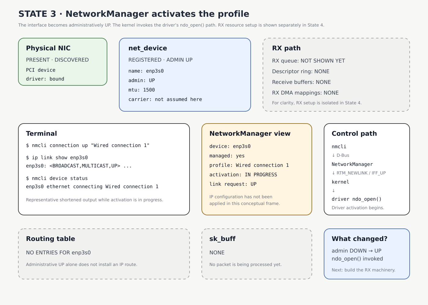
State 3 dashboard. NetworkManager has started profile activation, the kernel interface is now administratively UP, and the driver’s ndo_open() path has been entered. RX resources are intentionally postponed to the next frame, while routing and packet state remain empty.
The important distinction here is that UP is permission, not proof of connectivity. Linux has now allowed the interface to operate, but the driver still has to prepare the machinery that will actually let the NIC receive frames.
That is the next transition: building the RX queue, descriptor ring, receive buffers, DMA mappings, interrupt path, and NAPI state that connect the physical NIC to packet processing in the kernel.
Link transition: the Ethernet cable is plugged in
enp3s0 is already administratively UP because software enabled it in State 3. That does not mean a usable Ethernet link exists yet. Now we connect the cable. The PHYs at both ends can detect each other and establish the physical link, commonly using autonegotiation to agree on parameters such as speed and duplex where applicable.
Once the link is established, the NIC reports carrier to the driver and Linux can update the interface’s lower-layer and operational state. The administrative state does not change. In our simplified story the transition is therefore admin: UP → UP, carrier: DOWN → UP, and operstate: DOWN → UP. The ip link output makes this distinction visible in one place: UP inside the angle-bracket flags means the administrative IFF_UP flag is set, LOWER_UP means the lower layer reports carrier, while state UP is the interface’s operational state. Linux operational state documentation
Cable-connected dashboard
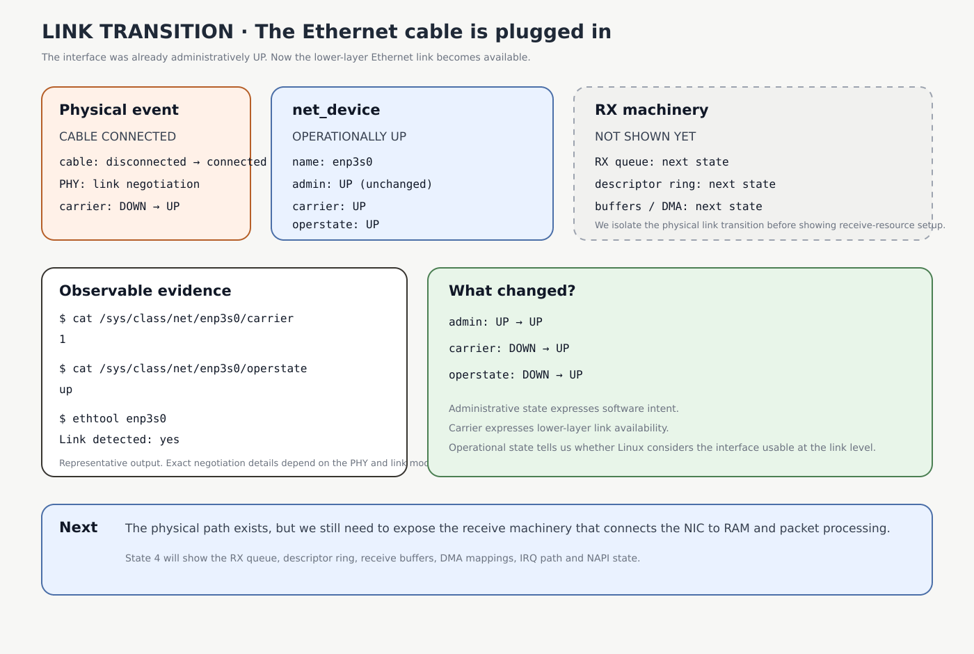
Link transition dashboard. The cable is now connected, carrier appears, and Linux can report the interface as operationally UP, while the administrative state remains UP.
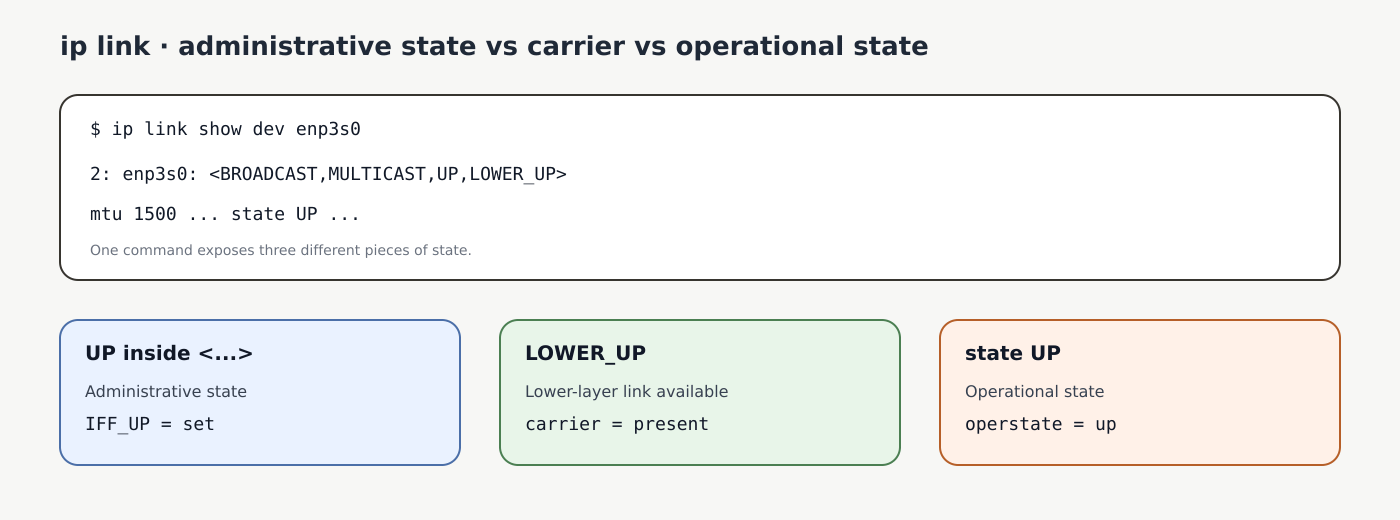
The ip link command makes the distinction visible in one place: UP inside the flags means the administrative IFF_UP flag is set, LOWER_UP reports lower-layer carrier, and state UP is the operational state.
This distinction is easy to miss but important: administrative UP means that software has enabled the interface, while operationally UP means that the lower-layer conditions needed for the interface to operate are available. With the physical link established, we can now return to the driver and expose the RX machinery that will actually move received frame data into RAM.
State 4: the driver builds the RX machinery
The interface is already administratively UP, but that alone is not enough to receive a frame. The driver still needs a concrete path between the NIC and RAM, which means preparing the RX queue, descriptor ring, receive buffers and DMA mappings, then wiring that path into interrupt handling and NAPI.
The important relationship is simple: the descriptor ring does not contain the Ethernet frames themselves. Its descriptors identify receive buffers that the NIC is allowed to use. Once those buffers are DMA-mapped and their addresses are programmed into the NIC, the hardware can place incoming frame bytes directly into RAM without the CPU copying each byte itself. The driver also prepares the notification path, typically using interrupts together with NAPI, so completed receive work can later be processed by the kernel. Linux DMA API documentation Linux NAPI documentation
The exact order is driver-specific. Some drivers allocate parts of this machinery during probe(), while others do more of it when the interface is opened through ndo_open(). Our dashboard shows the conceptual end state: the receive machinery exists and is ready before the first frame arrives.
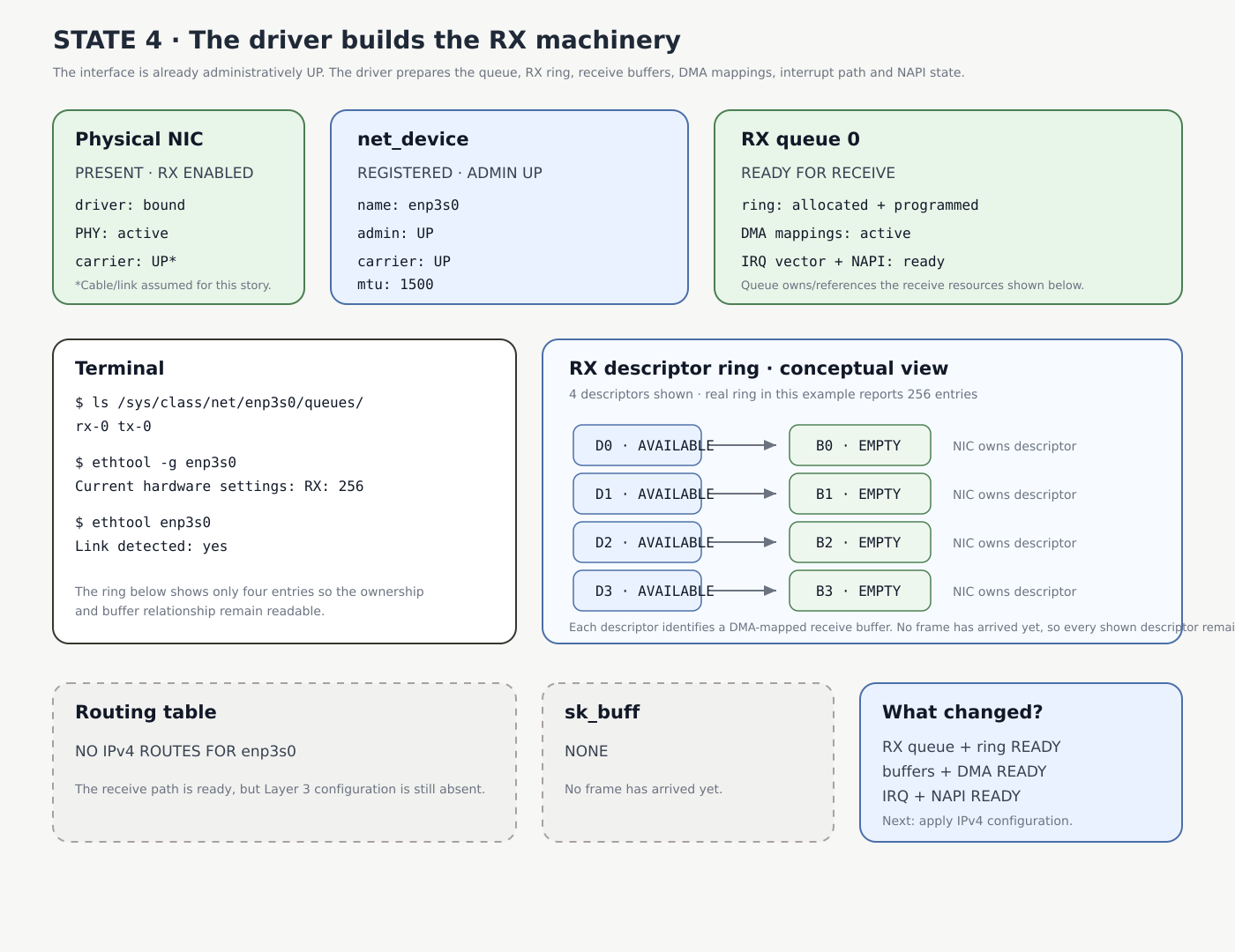
State 4 dashboard. The RX queue, descriptor ring, receive buffers, DMA mappings, interrupt path and NAPI state now exist. The NIC is ready to place incoming frame data into RAM, but no packet has arrived yet, so there is still no sk_buff.
At this point the machine has everything it needs at the device level to receive Ethernet traffic, but it still has no IPv4 identity in our story. The next transition adds that Layer 3 state.
State 5: the interface gets IPv4 configuration
To keep this part focused on the Linux networking stack rather than turning it into a DHCP walkthrough, we will use a static IPv4 profile. Our example address is 192.0.2.10/24 with 192.0.2.1 as the default gateway. The 192.0.2.0/24 network is reserved for documentation examples, which makes it safe to use here. RFC 5737
NetworkManager now applies the Layer 3 configuration from the active profile to the kernel. The address itself is not simply another field inside net_device; Linux keeps IP address state separately and associates it with the interface. Through rtnetlink, NetworkManager can add the address with an RTM_NEWADDR request and install routing state with RTM_NEWROUTE requests. rtnetlink documentation
In our simplified configuration, adding 192.0.2.10/24 gives the machine a connected route for 192.0.2.0/24 and a local route for its own address, while the gateway configured in the profile provides the default route through 192.0.2.1. These routes are not only configuration that we can inspect with ip route. They become input to the kernel's forwarding decisions when packets later enter IPv4 processing.
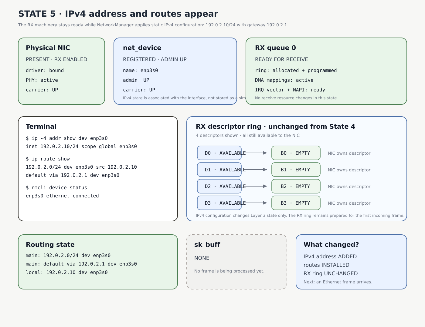
State 5 dashboard. The RX machinery remains ready, while NetworkManager has now applied static IPv4 configuration. The kernel contains 192.0.2.10/24, the connected and local routing state, and a default route through 192.0.2.1. There is still no sk_buff because no frame is being processed yet.
We have now finished the setup part of the story. The hardware exists, Linux has a net_device, NetworkManager has activated its profile, the receive machinery is ready, carrier is available, and Layer 3 configuration exists. The next state can finally start with the event we have been preparing for all along: an Ethernet frame arrives at the NIC.
State 6: an Ethernet frame arrives
Until now the receive machinery has been prepared but idle. We now let one Ethernet frame reach the NIC. The NIC selects an available RX descriptor, which in our simplified ring is D0, follows the DMA address associated with B0, and writes the frame bytes directly into that receive buffer in RAM.
Once the transfer is complete, the NIC marks the receive work as completed and signals the CPU through the configured interrupt path.
At this moment the driver has usually done two important things: it has acknowledged the receive event and it has suppressed further RX interrupts for that queue, handing control over to NAPI polling until the receive work is drained so that the completed RX entry can be processed outside the hard interrupt path. Linux NAPI documentation
There is an important boundary here: the Ethernet frame already exists in RAM, but Linux has not yet created an sk_buff for it. At this instant we still have hardware-facing receive state: one completed descriptor and one filled receive buffer. The higher-level packet object will appear only when the driver and NAPI process that completion in the next state.
Our ring remains deliberately simplified. Real NICs use different descriptor formats, ownership conventions and completion mechanisms, and some hardware separates submission and completion rings. The dashboard combines those details into one conceptual ring so that we can follow the lifecycle of one buffer without tying the explanation to a particular NIC.
State 6 dashboard
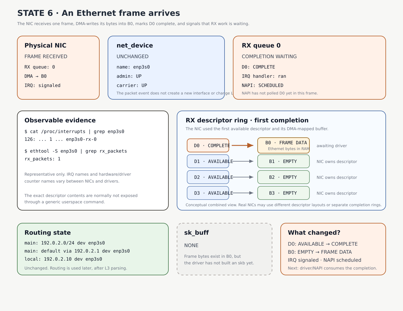
State 6 dashboard. The NIC has used D0 and DMA-written the incoming Ethernet frame into B0. D0 is now complete, B0 contains the frame bytes, the interrupt path has fired and NAPI is scheduled. D1–D3 remain available, and sk_buff is still absent because the driver has not consumed the completion yet.
This is the first moment in the story where actual packet bytes exist inside the machine. The next transition moves ownership back toward the CPU: NAPI polls the RX queue, the driver consumes D0, and Linux creates or builds the sk_buff that will carry the packet into the networking stack.
State 7: NAPI turns the completed receive into an sk_buff
In State 6 the interrupt handler scheduled NAPI, but that handoff has another important effect. Once NAPI owns the receive work, the driver should keep further interrupts for that NAPI instance masked until polling is finished, because another interrupt would only report work that the poller is already responsible for. Some devices mask the interrupt automatically, while other drivers do it explicitly before scheduling NAPI. The kernel documentation describes this as the normal NAPI scheduling pattern. Linux NAPI documentation
The driver’s NAPI poll() function now examines the receive ring and finds D0 complete. It obtains the packet data from the associated receive buffer, reads the metadata supplied by the NIC, and creates or prepares an sk_buff for the packet. The important point is that an sk_buff is primarily a metadata object. The packet bytes live in associated memory that the skb references, although individual drivers may instead copy some or all of the data into newly allocated skb storage. Linux sk_buff documentation
For our visualization we will follow one simple path: the packet data originating in B0 becomes the data referenced by the new skb, while the driver refills D0 with a fresh empty buffer, B4, so the RX ring can receive another frame. Real drivers may recycle the same page, copy small packets, use page pools, or manage completions differently, but the conceptual transition is the same: the completed receive resource is consumed, an skb is created, and the ring is replenished.
When the receive work has been drained, the driver can complete the NAPI cycle and allow RX interrupts again. We freeze the story immediately after the skb exists and the ring is ready again. In a real driver, the handoff into the generic receive path commonly happens inside the same NAPI poll callback, but keeping it for the next frame lets us see the boundary between the NIC/driver world and the generic Linux networking stack.
State 7 dashboard
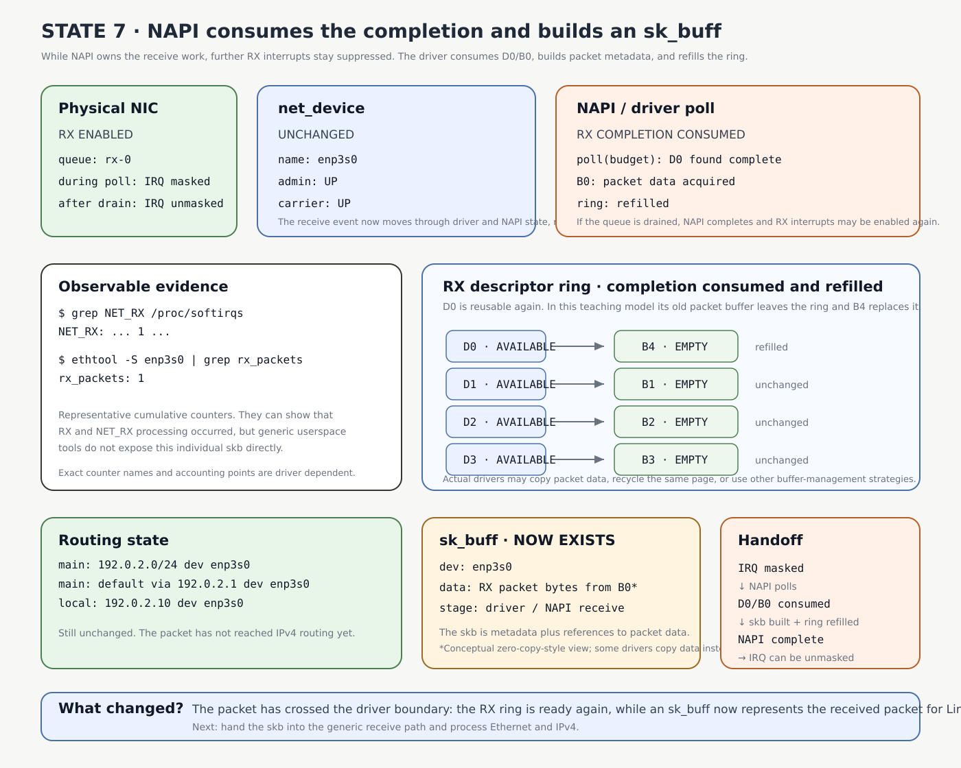
State 7 dashboard. NAPI consumes the completed D0 entry while RX interrupts are suppressed, the driver builds an sk_buff for the received packet, and the ring is replenished with a fresh empty buffer. Once the queue is drained, NAPI can complete and the RX interrupt can be enabled again.
At this point the packet has crossed an important boundary. The RX ring is back in a reusable state, while Linux now has an sk_buff that can move independently through the networking stack. The next state follows that skb into the generic receive path, where Ethernet and IPv4 processing begin.
State 8: the packet enters the generic Linux networking stack
We now resume the packet at the conceptual handoff point we deliberately separated from State 7. In real driver code this handoff normally happens inside the NAPI poll function, before that polling cycle completes, but treating it as a separate frame lets us see the moment when the packet stops being primarily a driver concern and becomes a generic Linux networking object.
Before Linux can choose a Layer 3 handler, the Ethernet information has to tell it what kind of payload the frame contains. Drivers commonly use eth_type_trans(skb, dev) while preparing the skb for the receive path. Conceptually, this moves the skb past the Ethernet header and records the resulting protocol in skb->protocol. For our packet, the Ethernet EtherType identifies IPv4, so the skb is marked as ETH_P_IP. The driver then hands it into the generic receive machinery, commonly through napi_gro_receive(). GRO can combine compatible packets as an optimization, but with the single packet in our story we can treat it as passing through unchanged. Linux sk_buff documentation
The generic receive path can now dispatch the packet to IPv4 processing. The IPv4 handler validates and interprets the IP header, including the destination address, and the routing subsystem performs a route lookup. Conceptually, this is where Linux consults its FIB, Forwarding Information Base, using the routing state we created earlier to determine what should happen next.
This lookup is one of the major branching points in the networking stack. If the destination belongs to this machine, processing continues toward local delivery. If the destination should be reached through another interface and forwarding is enabled, the packet can enter the forwarding path. If Linux cannot produce a usable route, processing can terminate instead.
Our packet is addressed to 192.0.2.10, which belongs to this host, so the lookup selects local delivery. We therefore continue toward TCP rather than following the forwarding path.
State 8 dashboard
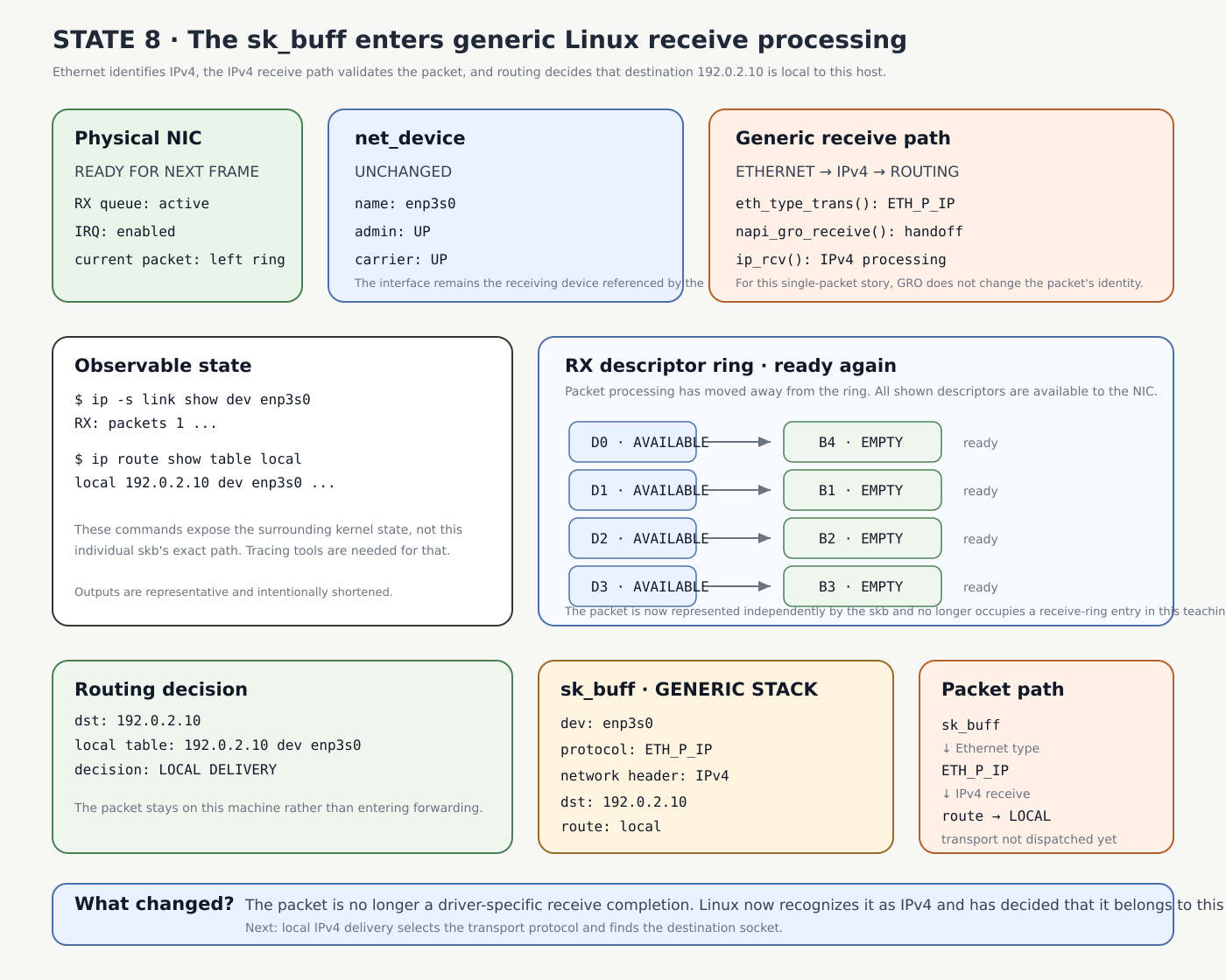
State 8 dashboard. The RX ring is reusable again while the sk_buff moves through the generic receive path. Ethernet processing identifies IPv4, IPv4 processing reads destination 192.0.2.10, and the routing subsystem selects LOCAL DELIVERY. The packet has not yet been dispatched to a transport protocol or socket.
The important change is that the packet now belongs to the generic networking stack rather than to the NIC receive machinery. From this point onward, the RX ring can receive completely different frames while this skb continues independently toward the application. The next transition is local IPv4 delivery, where Linux reads the IP protocol field, enters the appropriate transport implementation, and begins looking for the destination socket.
State 9: TCP finds the established socket
State 8 ended when IPv4 routing decided that the packet belongs to this machine. Local IPv4 delivery can now inspect the IP Protocol field to decide which transport implementation should receive the packet. For our packet the value is 6, which means TCP, so Linux passes the sk_buff into the TCP receive path, conceptually through a handler such as tcp_v4_rcv().
To keep this journey focused on the receive path rather than turning it into an explanation of the TCP handshake, we will assume that a connection already exists. Our local application has an established TCP socket on 192.0.2.10:8080, connected to a peer at 192.0.2.20:51514, and the segment we are following contains in-order application data.
This is where ports finally become part of the routing of the packet inside the machine. IP routing brought the packet to the local host, but it did not decide which application should receive it. TCP now uses the connection identity, commonly described by the four values source IP, source port, destination IP, and destination port, together with TCP connection state, to find the matching established socket. socket(7)
Once the socket has been found, TCP processes the segment according to the state of that connection, including its sequence and acknowledgement information, receive-window state, and checksum status as required. In our simple case the payload is the next expected in-order data, so TCP can accept it and place the received bytes into the socket’s receive state. If the application is sleeping while waiting for data, Linux can wake it.
There is another important abstraction change here. The application will not receive an Ethernet frame, an IP packet, or an sk_buff. TCP presents an ordered byte stream. The packet boundaries that were so important in the lower layers are no longer the interface that userspace sees. We therefore stop this state with data waiting on the established socket, just before the application calls recv() or read().
State 9 dashboard
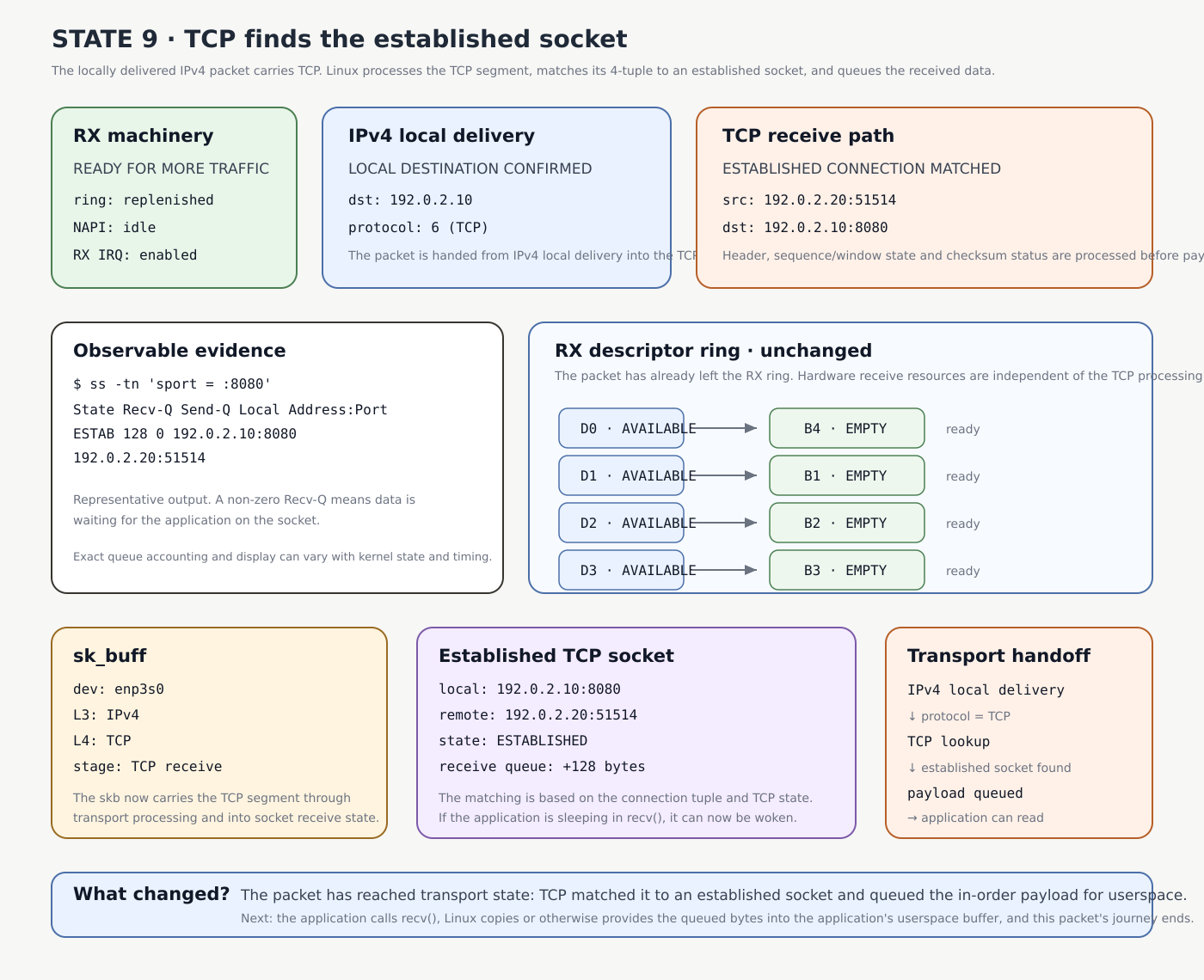
State 9 dashboard. IPv4 local delivery identifies TCP, the TCP receive path matches the segment from 192.0.2.20:51514 to the established socket at 192.0.2.10:8080, and the accepted in-order payload is queued for the application. The RX ring remains reusable and independent of this transport processing.
At this point the networking stack has answered the last kernel-side addressing question: not only does the packet belong to this machine, it belongs to this particular TCP connection and socket. The final transition is the boundary we have been moving toward from the beginning: the application calls recv(), and the queued TCP bytes cross from kernel-managed socket state into the application’s userspace buffer.
State 10: the application receives the TCP byte stream
State 9 ended with 128 bytes waiting in the receive state of our established TCP socket. The networking stack has already done the work needed to decide where those bytes belong, but they are still kernel-managed data. The application has not received them yet.
The final transition begins when the application calls something such as recv(fd, buf, 4096, 0). That call crosses the userspace-to-kernel boundary and asks the socket layer to provide bytes that TCP has made available on this connection. For a normal copied receive path, Linux copies available stream data from the socket’s receive state into the buffer supplied by the process. recv(2) / recvmsg(2) documentation
For our simplified example, the application’s buffer is larger than the 128 bytes waiting on the socket, so one recv() call consumes all of them and returns 128. The socket itself remains established. What changes is the data ownership: the receive queue drops from 128 bytes to 0, while the process now has those 128 bytes in its own userspace memory.
A real TCP read does not have to line up with the segment that originally carried the data. recv() may return fewer bytes than requested, multiple TCP segments may contribute to one read, and one segment’s data may be consumed across multiple reads. That is exactly the point of TCP’s byte-stream abstraction. In our one-packet teaching path, however, we deliberately consume the entire payload at once so that the final lifecycle transition remains visible.
Once all data associated with our packet has been consumed and nothing else still references that packet storage, the corresponding sk_buff and backing resources can be released or recycled. The application never sees that cleanup. From its point of view, recv() simply returns bytes.
State 10 dashboard
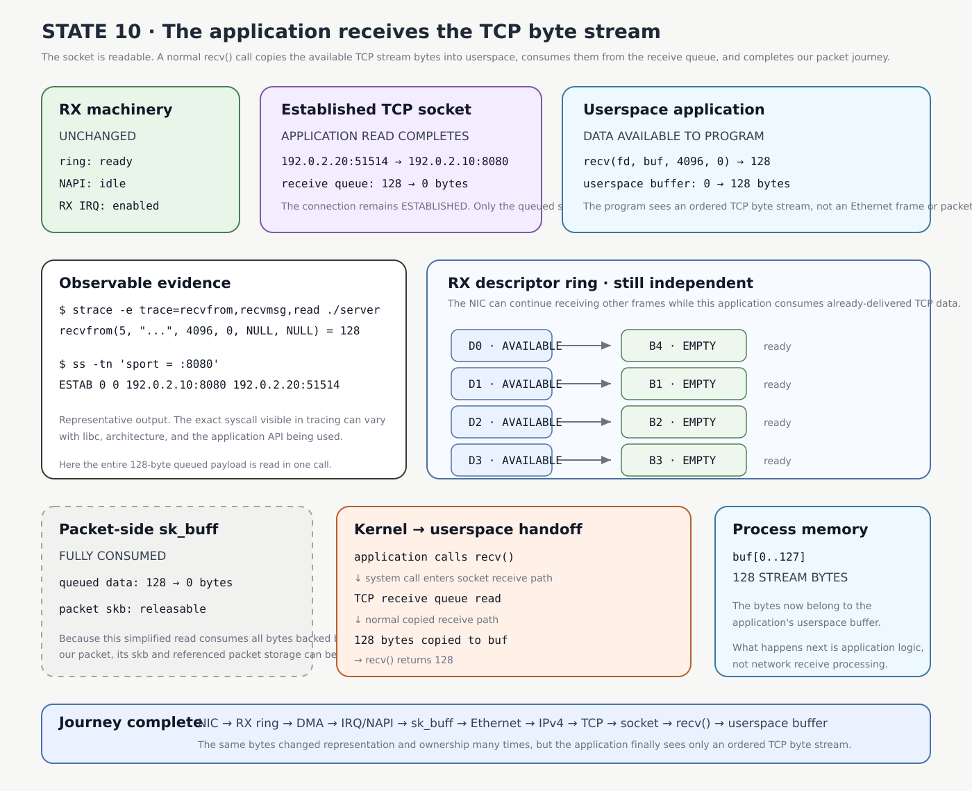
State 10 dashboard. The application calls recv(), the established socket’s receive queue goes from 128 bytes to 0, and those 128 bytes appear in the process’s userspace buffer. The RX ring remains ready for unrelated traffic, while the packet-side sk_buff can be released once its data has been fully consumed.
That completes the journey. The same network data began as an electrical or optical signal outside the machine, became bytes in a DMA receive buffer, passed through descriptor and NAPI processing as an sk_buff, moved through Ethernet, IPv4 and TCP, waited on a socket, and finally became ordinary bytes in a userspace buffer.
The most useful lesson is not the exact function sequence, because drivers, kernel versions, offloads and configuration can change many details. It is the sequence of representations, ownership changes and boundaries. The NIC does not write directly into an application’s buffer, the driver does not hand Ethernet frames directly to a process, and TCP does not expose packets to the application. Linux repeatedly transforms the same underlying data until the abstraction visible to the program is simply an ordered stream of bytes.
And what about sending?
The transmit path reuses many of the same actors, but it is not simply the receive path played backward. On receive, hardware introduces the data into the machine and Linux gradually turns it into something an application can consume. On transmit, the application already owns the bytes, and the kernel gradually turns them into something the hardware can put onto the link.
Suppose our application calls send() or write() on the established TCP socket. TCP accepts those bytes into the outgoing stream and prepares the transport data that must be transmitted. IPv4 processing and routing then determine the outgoing path, while the lower networking layers prepare the packet for the selected interface. Before the driver sends it to hardware, the packet will typically pass through the interface’s egress queueing machinery, where Linux can queue and schedule transmission.
The driver then prepares the hardware-facing side. It DMA-maps the packet memory as required, places references to that memory into TX descriptors, and makes the descriptors available to the NIC. This time the DMA direction is the opposite of receive: instead of the NIC writing incoming bytes into RAM, the NIC reads packet data from RAM and transmits the resulting Ethernet frame onto the link. After the hardware finishes, it reports completion so the driver can reclaim TX descriptors and release or recycle resources. Offloads can move work such as checksum calculation or segmentation into the NIC, but they do not change this basic ownership flow. Linux network device driver documentation Linux DMA API documentation
Short transmit-path view
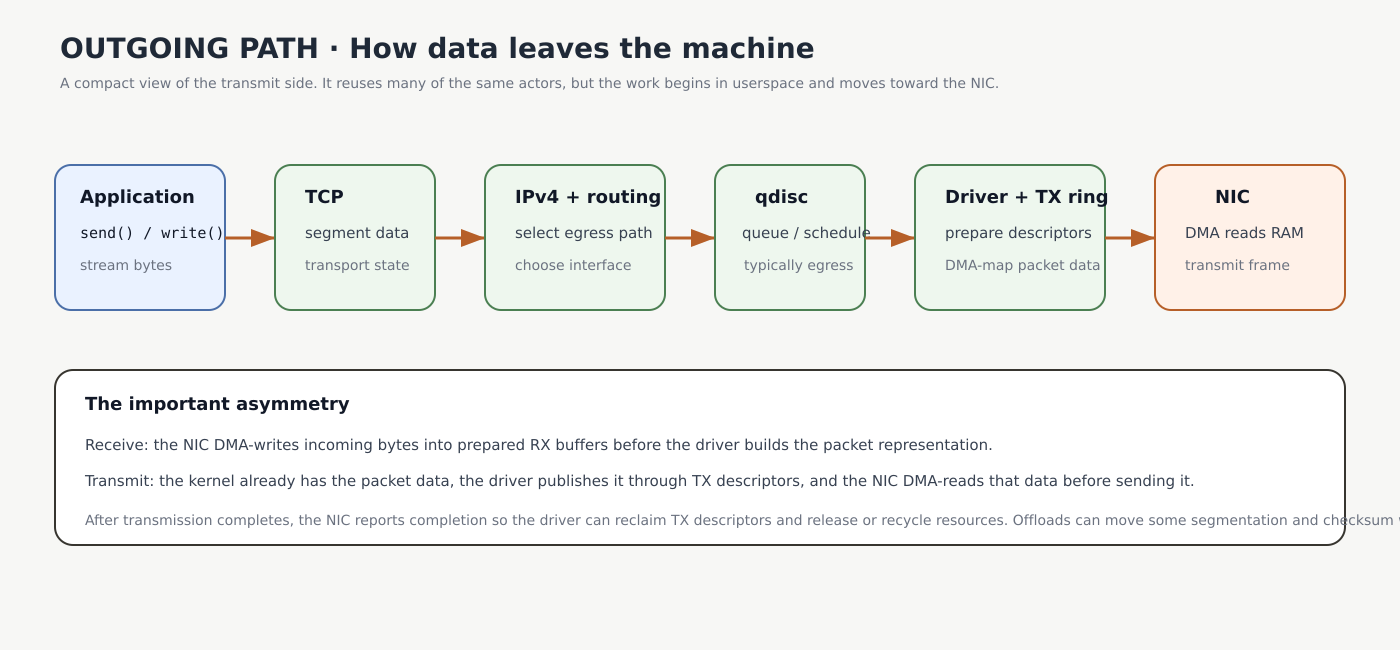
Transmit-path overview. Application bytes move through the socket and protocol stack toward the egress interface, the driver publishes packet memory through the TX ring, and the NIC DMA-reads that memory before putting the frame onto the link.
We could follow every TX transition with the same level of detail as the receive path, including queueing disciplines, neighbor resolution, offloads and completion handling. For this article, that would mostly repeat machinery we now already recognize. The important addition is the direction of ownership: receive starts at the NIC and ends in userspace, while transmit starts in userspace and ends at the NIC.
Summary
We did not cover every possible branch through the Linux networking stack. We did not follow forwarding or dropping packet by packet, and the transmit path above is intentionally only a compact overview rather than another full sequence of states.
But we did cover the main machinery that makes the stack work: the NIC and driver, administrative and operational link state, RX queues and descriptor rings, DMA, interrupts and NAPI, sk_buff, Ethernet and IP processing, routing, TCP, sockets, userspace delivery, and finally the shape of the path back out of the machine.
Forwarding, dropping and the detailed transmit path add their own decisions, queues and protocol-specific behavior, but they build on the same machinery. Once these objects, boundaries and ownership transitions are clear, the rest stops looking like a completely different system.
What is next
In the final part of this series, we will look at how one physical machine can become an entire network by using Linux virtualization tools.
We will take the networking machinery we have already built and use virtual interfaces, network namespaces, and related Linux primitives to create multiple isolated hosts and connect them together inside one system.
Sources
Understanding Linux Network Internals by Christian Benvenuti
Linux Kernel Networking: Implementation and Theory by Rami Rosen
Assistance
ChatGPT, GPT-5.6 Sol
Series Hub:
Networking in the Power Grid for Software Developers

I have worked with networked software for years, but for most of that time the network was something I used rather than something I really understood. I could open a socket, call an API, connect to an IP address, and continue with the part of the system I was responsible for.